
Today we will look at the concept of linear regression.
The dictionary meaning of regression means “return to the origin state.”
The term begins with the British geneticist Francis Galton studying the laws of inheritance. In studying the relationship between parents and children’s heights, Galton surveyed and tabulated the averages of heights of fathers and mothers. I found it. Galton called it a regression analysis.
Let’s say we have the following data:
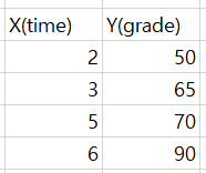
The effective range of scores predicted from the above data is between 0 and 100 points.
When training with the above data, that is, training data set,
A model is created that is the basis of the corresponding regression model.
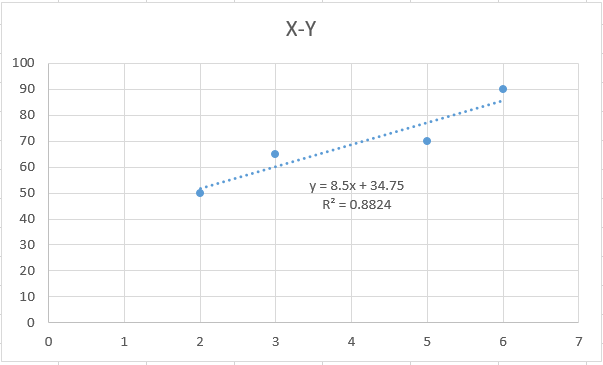
The linear regression method finds the best model, such as when the distribution of data can be represented by a straight line. We assume that the model of the data we have learned is correct, and we can learn that finding and representing this straight line. When graphing with data from Excel, getting a trendline is the basic example of linear regression.
In terms of the formula,
H (x) = Wx + b
H (x) represents our hypothesis, and the shape of the line depends on the value of W (Weight) and the value of b (bias).
The hypothesis for the data set above can be expressed as H (w) = 1 * x + 0 (because the axis started at zero).
Here, it can be seen that the drawn line calculates the difference from the distribution of each data so that the smallest line is suitable for this model.
So this is called cost function. This cost function allows us to gauge how different our hypothesis is from what we actually represent.
Borrowing the simple expression above, you can’t really find out how different the value is. This is because the above form can only be calculated when the difference is given and given a representation of the actual value that is greater than the hypothesis data.
To represent this, we take the square of the equation. Based on this, these weights can be automatically assigned to actually give more penalties to larger values. The formula for the cost function is as follows.

In general, if m is the number of data, the result is equal to the total number of data of the squared difference between the predicted value X and the actual data value Y. will be. As a result, this linear regression finds the value of W (weighted) and finely adjusted b (bias) when the line is drawn on the graph to find the minimum value of silver with the smallest difference between the hypothesis and the actual data. It can be seen as the learning of linear regression in learning.