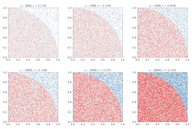
The Monte Carlo method is a term for an algorithm that probabilistically calculates the value of a function using random numbers. Frequently used in mathematics and physics, it is used to approximate calculations when the value to be calculated is not represented in closed form or is complex. Stanislaw Ulam is named after Monte Carlo, Monaco’s famous gambling city.
In 1930, Enrico Fermi was famous for using this method to study the properties of neutrons. He also played a key role in the simulation of the Manhattan plan and the development of hydrogen bombs.
Because of the iteration of the algorithm and the large number of calculations involved, Monte Carlo is suitable for computer calculations using various computer simulation techniques.
The Monte Carlo method (or Monte Carlo experiment) is a wide range of computer algorithms that uses a method of random sampling repeatedly to obtain mathematical results. The idea behind this algorithm is to use randomness to solve problems that may be deterministic. This method is usually used to solve physics or mathematics problems and is most useful when no other directions are available. The Monte Carlo method is mainly used for optimization, numerical integration, and derivation from probability distributions.
In physics problems, the Monte Carlo method is useful for simulating systems with many degrees of freedom of binding, such as fluids, disordered materials, strongly bonded solids, and cellular structures. Other examples include modeling phenomena with significant uncertainty in input values, such as business risk calculations, and multidimensional static components with complex boundary conditions in mathematics. In application to system engineering problems (space, oil exploration, aircraft design, etc.), failure prediction, cost overruns and schedule overruns based on Monte Carlo methods are routinely better than human intuition or alternative methods.
The goal in other problems is to derive from a series of probability distributions that satisfy nonlinear evolutionary equations. This flow of probability distributions can be interpreted as a distribution of random states in the Markov process, where the transformation probability always depends on the distribution of the current random states.
These models can also be seen as the evolution of the law of random states of nonlinear Markov chains. A representative way to simulate this sophisticated nonlinear Markov process is to sample many copies of the process, replacing the unknown distribution of random states in the evolutionary equation with a sampled empirical scale. In contrast to traditional Monte Carlo and MCMC methodologies, this average field particle technique relies on sequential interaction samples. The term average field reflects the fact that each sample interacts with the empirical measure of the process. When the size of the system tends to be infinite, these random measurements converge into a deterministic distribution of random states of the nonlinear Markov chain, thus eliminating statistical interactions between the particles.

import numpy as np

plt.figure(figsize=(10,6))
plt.plot(x[idx == 0], y[idx == 0], 'b.')
plt.plot(x[idx == 1], y[idx == 1], 'r.')
plt(axis('equal')
plt.show()

pi = np.sum(np.abs(x + 1j*y) < 1)/n *4

print(pi)
