
After the release of Perceptron in 1958, the New York Times published a shocking article on the 8th of July that a computer would be developed that would soon walk, speak, and recognize self. But in 1969, Marvin Minsky devised a multilayer perceptron (MLP) to solve the XOR problem, and said there is no way to learn MLP.
As I mentioned earlier, in 1974, Dr. Paul Werbos, a Ph.D. student at Harvard University, gave a dissertation on how to learn MLP, which is ignored by Marvin Minsky. The key method of the paper is the error backpropagation algorithm.
Back propagation
The back propagation algorithm is the most basic and general algorithm for learning ANN, artificial neural network, and ANN. Backpropagation is a name given because an error is propagated in the opposite direction of the original direction.
The two steps of the algorithm are:
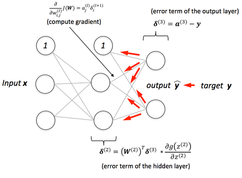
1. Forward training is performed by inserting training data as input. Calculate an error that differs from the resulting Neural Networks Prediction value and the actual Target Value.
2. Backpropagate an Error to each Node of Neural Networks.
Characteristics of Backpropagation Algorithm
Backpropagation algorithms are a way of learning neural networks with known inputs and outputs (called supervised learning). There are a few things you need to know about MLP before applying the backpropagation algorithm.
Initial weights and weights are given randomly.
Each node is considered a perceptron. In other words, the active function is applied whenever the node passes by. We will call the net before the active function and out. The out value is used to calculate the next layer. The last out is the output.
The activity function is the sigmoid sigmoid function. (This function is typical because it is easy to differentiate, but you can use other active functions instead of other active functions.)
If we target the value we want to get as the result, and the output we get is the output, the error E is Here, sum means adding up all the errors that occur in all outputs (output1, output2…). The final goal is to approximate the value of the function E for this error to zero. When the error approaches zero, the neural network will produce the output we want, the correct answer for the inputs used for learning and similar inputs.

Plot error E with two weights each. E is minimum when y = 0, w1, w2 = 0 on the graph. (Wikipedia) Error E with all weights w1… From the equation for wn, what we need to do is modify the weight w so that E is minimum.
To do this, we use an optimization algorithm called gradient descent. The basic principle is to continuously move toward the lower slope to reach the point where the value is minimum (extreme value).
To this end, a process of differentiating the error E is required. Since all weights affect the error E, the E is divided into the respective weights. In a multilayer neural network, each layer is connected so that the value used in the differential process close to the output is used in the differential process far from the output. Therefore, the derivative closest to the output is processed first.