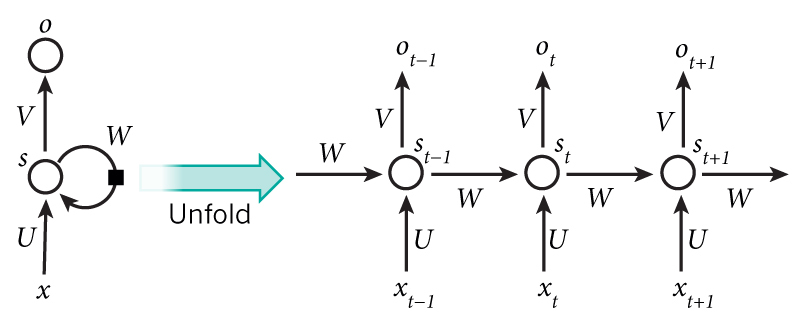
Neural networks that process sequential data must have three functions:
Temporality: Features must be entered one at a time in order.
Variable length: To process a sample of length n, the hidden layer must appear n times.
Context dependency: Remember the previous feature and use it at the right moment.
To design a learning model with all of these features, you can extend the MLP a bit.
Structure of RNN
The structure of the circulatory neural network is similar to that of MLP. RNN has an input layer, a hidden layer, and an output layer. It should be noted that there is only one hidden layer. Another thing to note is that unlike MLP, there are edges between hidden nodes. These edges are called circular edges because they connect the hidden and hidden nodes. RNNs have circular edges and thus have all three functions: temporal, variable length, and context dependent.
When multiple nodes are abbreviated as layers, the black squares attached to the circular edges of the hidden layer indicate that the neural network operates over time. That is, it calculates at time 1, takes the result at time 2, and calculates at the time 3 with the result, repeating the length of the sequential data.
This time connectivity can be expressed by the following equation. This expression explicitly shows that RNN calculates based on the value of the parameter. Theta is the set of weights of the RNN. It is shown that the hidden layer value of the instant t is determined by the input value of the instant t and the hidden layer value of the immediately preceding instant.
The hidden layer of the RNN is responsible for ‘remembering’ previous information. Therefore, the hidden layer node of the RNN is called a ‘state’ variable.
If you look at the RNN structure, you’ll see that the parameters, or weights, are ‘shared’. Over time, a new vector is input and calculated using weights, using the same weight each time.
Weight sharing has several advantages. First, it significantly reduces the number of parameters to be estimated by the learning process, keeping the optimization problem at a reasonable size. Second, the number of parameters is constant regardless of the length of the feature vector. Third, the same or similar output can be produced even if the moment the feature appears is reversed.
Operation
Once you understand the structure of RNN, you can easily understand its behavior. RNNs have similar behavior as MLPs, but they update the state of the neural network and compute a vector h that represents the entire hidden layer.
After calculating the hidden layer, the output layer is calculated and the final output is usually determined by applying the softmax function to the active value.


