Last time, we even learned a hierarchical clustering algorithm. This time, let’s look at an algorithm called DBSCAN (Density-based spatial clustering of applications with noise).
DBSCAN is a very useful clustering algorithm, and its main advantage is that you do not need to specify the number of clusters in advance. This algorithm can also find complex shapes, and can identify points that do not belong to any class. DBSCAN is somewhat slower than merged clusters or k-means, but can be applied to relatively large datasets.
DBSCAN finds points in a crowded area with lots of data in the characteristic space nearby. This region is called the dense region of the characteristic space. DBSCAN’s idea is that dense clusters of data make up one cluster and are clustered with other clusters around relatively empty areas.
Parameters – min_samples, epsilon
Points in dense regions are called core sample points and are defined as follows. DBSCAN has two parameters min_samples(min_points) and eps(epsilon). If the number of min_samples is contained within the eps distance from a data point, the data point is classified as a core sample. Core samples closer than eps are merged into the same cluster by DBSCAN.
Algorithm
This algorithm randomly picks points at startup. It then finds all points within the eps distance from that point. If the number of points in the eps distance is less than min_samplse, the point is labeled with noise that does not belong to any class. If there are more points in the eps distance than min_samples, the points are labeled as the core sample and a new cluster label is assigned. Then look at all the neighbors of that point. If the points is a core sample, visit the point’s neighbors one after another. By continuing in this way, the cluster grows until there are no more core samples within the eps distance. Then, select points that have not been visited and repeat the process.
If not assigned to any cluster, assign the cluster label you just created.
In the figure below, if minPts = 4, if there are 4 or more points in the epsilon radius around the blue dot P, it can be judged as one cluster. It becomes the core point.
In the figure below, in the case of the gray point P2, since there are 3 points in the epsilon radius based on the point P2, it does not reach minPts = 4, so it is not the core point that becomes the center of the cluster, but the previous point P is the core point. This is called a boder point because it belongs to the cluster.
In the figure below, P3 becomes the core point because it has 4 points within the epsilon radius.
However, another core point P is included in a radius centered on P3, and in this case, core points P and P3 are said to be connected and are grouped into one cluster.
P4 in the figure below is not included in the range that satisfies minPts = 4 no matter what the point is. In other words, it becomes an outlier that does not belong to any cluster, which is called a noise point.
Example codes
import pandas as pd
import numpy as np
import matplotlib.pyplot as plt
import seaborn as sns
from sklearn.cluster import DBSCAN
from sklearn import datasets

data1 = np.load('./data/outlier2.npy')

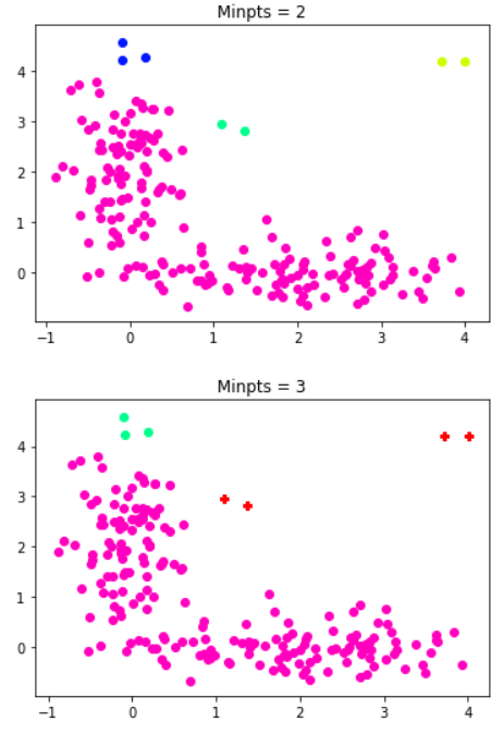
for minpts in [2,3]:
    fig = plt.figure()
    plt.title('Minpts = '+str(minpts))
    dbscan1 = DBSCAN(eps = 0.5, min_samples = minpts)
    dbscan_result1 = dbscan1.fit_predict(X = data1)

    if -1 in dbscan_result1:
        k = np.size(np.unique(dbscan_result1))-1
        noise_list = data1[dbscan_result1 == -1]
        plt.scatter(noise_list[:,0],noise_list[:,1],color='r', marker='P')
    else:
        k = np.size(np.unique(dbscan_result1))

    NUM_COLORS = k
    cm = plt.get_cmap('gist_rainbow')

    for i in range(k):
        i_cluster_list = data1[dbscan_result1 == i]
        plt.scatter(i_cluster_list[:,0],i_cluster_list[:,1],color=cm(1.*(k-i)/NUM_COLORS))


