The Gaussian distribution is another name for the normal distribution. The Gaussian distribution, widely known in statistics, is a very important concept. Last time, I mentioned the concept of probability and statistics and mentioned the central limit theorem. Let’s look at the central limit theorem again.
Central limit theorem
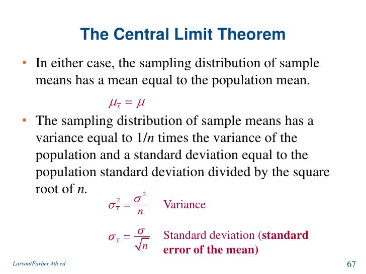
The sample data sampled from a population with a finite variance has the form of a normal distribution as the size of the sample data increases. That is, as n increases to an infinite value, it approaches the normal distribution.
Blind spots of central limit theorem: Assuming that the central limit theorem is convergent and that all situations converge to a normal distribution. In the case of insufficient domain data or special domains, it may not converge to the normal distribution.
The core of the central limit theorem is that as n increases, it follows the Gaussian distribution.
Gaussian Distribution
In probability theory, a normal (or Gaussian or Gauss or Laplace–Gauss) distribution is a type of continuous probability distribution for a real-valuedrandom variable. The general form of its probability density function is
The parameter mu is the mean or expectation of the distribution (and also its median and mode); and sigma is its standard deviation. The variance of the distribution is sigma^2. A random variable with a Gaussian distribution is said to be normally distributed and is called a normal deviate.
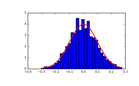
Now, let’s extract samples using the probability density function of the Gaussian Distribution function using python code.
The python code is shown below.
import numpy as np
import matplotlib.pyplot as plt

mu, sigma = 0, 0.1 # mean and standard deviation
s = np.random.normal(mu, sigma, 1000)
abs(mu - np.mean(s)) < 0.01
abs(sigma - np.std(s, ddof=1)) < 0.01

count, bins, ignored = plt.hist(s, 30, normed=True)
plt.plot(bins, 1/(sigma*np.sqrt(2*np.pi))*np.exp(-(bins - mu)**2/(2*sigma**2) ),linewidth=2, color='r')
plt.show()

The Gaussian distribution belongs to the family of stable distributions which are the attractors of sums of independent, identically distributed distributions whether or not the mean or variance is finite. Except for the Gaussian which is a limiting case, all stable distributions have heavy tails and infinite variance. It is one of the few distributions that are stable and that have probability density functions that can be expressed analytically, the others being the Cauchy distribution and the Lévy distribution.
Original Model is a commonly used algorithm. And there is a feature that needs to create a new featrure using existing features. This can be risky if you have to create it yourself. It is necessary to analyze the problem through error analysis and solve it.
However, it is easy to process a lot of data because the computational cost is low. Even if the number of features n is as large as 100,000, there is no burden to perform. It is because of these advantages that it is commonly used.
Also, it works well even if the training set is small. Anomaly detection is possible with only about 100 datasets.


Appreciating the time and energy you put into your blog and detailed information you
present. It’s nice to come across a blog every once in a while that isn’t the same outdated rehashed material.
Excellent read! I’ve bookmarked your site and I’m adding your RSS feeds to my Google account.
WOW just what I was looking for. Came here by searching for
g and
I could not refrain from commenting. Very well written!
I’d like to thank you for the efforts you have put in penning this blog.
I’m hoping to check out the same high-grade blog posts
from you in the future as well. In fact, your creative writing abilities has encouraged me to get
my own, personal site now 😉
I love your blog.. very nice colors & theme. Did you design this website yourself or did you hire
someone to do it for you? Plz respond as I’m looking to construct my
own blog and would like to find out where u got this from.
appreciate it
Your style is really unique compared to other people I have read stuff from.
Thanks for posting when you have the opportunity, Guess I will just bookmark this site.
Wow, this piece of writing is fastidious, my sister is analyzing
such things, thus I am going to inform her.
It’s hard to find well-informed people in this
particular subject, but you seem like you know what you’re talking about!
Thanks
Woah! I’m really loving the template/theme of this website.
It’s simple, yet effective. A lot of times it’s difficult to get that “perfect balance”
between superb usability and visual appeal. I must say you’ve done a excellent job with
this. Additionally, the blog loads extremely fast for me on Internet explorer.
Excellent Blog!
Do you think so? Well I don’t think that my work is excellent. Anyway thanks