2020.03.29(pm): Statistical Inference and Hypothesis Testing

This time, let’s look at the concepts of probability and statistics that are the basis of machine learning algorithms.

When learning a model in the area of ​​supervised learning, the most important thing is variable selection. Numerical interpretation and verification are required to ensure good selection of this variable. So, what is needed is the establishment of hypotheses for variables, tests and judgments. After hypothesizing that a variable is a meaningful variable, it should be tested in a statistical way.

Before checking whether the hypothesis is correct or not, let’s look at the concepts of the null hypothesis and the alternative hypothesis.

Null hypothesis vs Alternative hypothesis

The null hypothesis(H₀) is a hypothesis subject to direct testing. For example, the hypothesis is, “A person who gets up early in the morning will have a lower life satisfaction.” The null hypothesis is an unproven claim or hypothesis. First, the whole process begins with the assumption that this null hypothesis is correct. Conversely, it is a hypothesis that since it is unlikely to be true, it is expected to be discarded from the beginning. In other words, the null hypothesis is aimed at rejecting it.

The alternative hypothesis(H₁) is an alternative to the null hypothesis. That is, the hypothesis is accepted when the null hypothesis is rejected. The alternative hypothesis is a new claim or a hypothesis that you really want to prove. In other words, the alternative hypothesis is to adopt.

p-value

There should be a ‘p-value’ for whether the null hypothesis is adopted or rejected, and this threshold is called a threshold. In the description of this threshold, the concept of ‘significance level‘ emerges. The ‘significance level’ is an error to reject even if the null hypothesis is actually right. To put it more easily, it’s a risk that comes with dismissing the null hypothesis. The null hypothesis is actually correct, but the probability of being wrong (risk) is called the significance level.

If the p-value is too low, the null hypothesis is rejected because the probability of a hypothesis is too low. Usually, the standard is decided, but in general social statistics, it is based on 0.05 or 0.01.

type I error vs type II error

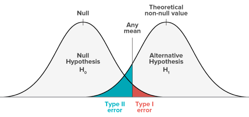
Type I error
If the null hypothesis is true, if you dismiss it, you are making a Type I error. The probability of making a Type I error is α, which is the significance level set for the hypothesis test. If α is 0.05, you acknowledge that there is a 5% chance of rejecting the null hypothesis incorrectly. To lower this risk, lower α values ​​should be used. However, using a lower alpha value is less likely to detect actual differences that actually exist.

Type II error
If the null hypothesis is false and you do not reject it, you are committing a second kind error. The probability of making a Type II error is β, which depends on the power of the test. By setting the power sufficient, you can reduce the risk of making a Type II error. Just make the sample size large enough to detect the actual difference.

t-test

This is a method to test whether the two groups have the same average. Normality and isovariance should be assumed. If normality is assumed (n> 30), a Z-test may be conducted. Generally, t-test is used when the sample is less than 30.

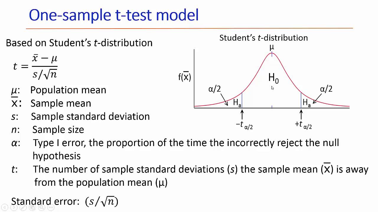
Z-test is sometimes used because more than 30 samples satisfy the central limit theorem. The Z-test is to use the actual population standard deviation, unlike the t-test using the sample standard deviation. If the same data is analyzed by year, the paired T-test should be tested.

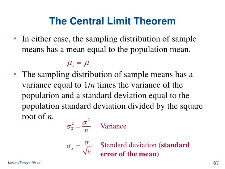
Central limit theorem

The sample data sampled from a population with a finite variance has the form of a normal distribution as the size of the sample data increases. That is, as n increases to an infinite value, it approaches the normal distribution.

Blind spots of central limit theorem: Assuming that the central limit theorem is convergent and that all situations converge to a normal distribution. In the case of insufficient domain data or special domains, it may not converge to the normal distribution.

The law of large numbers: When a trial with a certain probability is repeated in large numbers, the result of the event converges to the average value. For example, if you flip a coin with the front and back faces multiple times, the ratio will converge 1: 1.

Universal Approximation Theorem: A concept that can be said to be the central theorem in deep learning. It is a simple theory that all possible functions f (x) can necessarily converge into an artificial neural network. It is a concept often emphasized by many celebrities who study deep learning.

Hypothesis test(t-test) python code

import pandas as pd
import numpy as np

df = pd.read_csv('grades.csv')
print(len(df))
# 2315

early = df[df['assignment1_submission'] <= '2015-12-31']
late = df[df['assignment1_submission'] > '2015-12-31']

print(early.mean())
'''
assignment1_grade    74.972741
assignment2_grade    67.252190
assignment3_grade    61.129050
assignment4_grade    54.157620
assignment5_grade    48.634643
assignment6_grade    43.838980
dtype: float64
'''

print(late.mean())
'''
assignment1_grade    74.017429
assignment2_grade    66.370822
assignment3_grade    60.023244
assignment4_grade    54.058138
assignment5_grade    48.599402
assignment6_grade    43.844384
dtype: float64
'''

from scipy import stats

t_test1 = stats.ttest_ind(early['assignment1_grade'], late['assignment1_grade'])
print(t_test1)


#refer: https://engkimbs.tistory.com/758