2020.04.12(pm): Regression Example: Housing price prediction

This is a summary of Deep Learning Chapter4 from the founder of Keras.

This time, as an example of a regression problem, we will try to predict the housing price. The data we will use today is the Boston Housing Price Dataset, which estimates the median value of housing prices given data such as crime rates and local tax rates outside Boston in the mid-1970s. There are 504 data points, 404 training samples, and 102 test samples. Each feature in the input data has a different scale. Some values ​​appear as floats and some have integers.

Data download

First, let’s load the dataset in keras.

import keras
from keras.datasets import boston_housing

(train_data, train_targets), (test_data, test_targets) =  boston_housing.load_data()

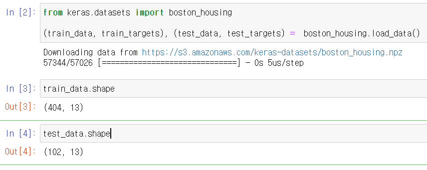
train_data.shape
test_data.shape

You can see the number of training data and test data as below. 13 means there are 13 numerical characteristics.
The 13 characteristics are:

1. Per capita crime rate.
2. Proportion of residential land zoned for lots over 25,000 square feet.
3. Proportion of non-retail business acres per town.
4. Charles River dummy variable (= 1 if tract bounds river; 0 otherwise).
5. Nitric oxides concentration (parts per 10 million).
6. Average number of rooms per dwelling.
7. Proportion of owner-occupied units built prior to 1940.
8. Weighted distances to five Boston employment centres.
9. Index of accessibility to radial highways.
10. Full-value property-tax rate per $10,000.
11. Pupil-teacher ratio by town.
12. 1000 * (Bk – 0.63) ** 2 where Bk is the proportion of Black people by town.
13. % lower status of the population.

The target is the median price of the house, in thousands of dollars.

Data preparation

Problems arise when injecting values ​​with different scales into a neural network before learning. The likelihood of making learning more difficult increases. Therefore, it is a typical method to normalize for each feature before training the data. Below is the code that subtracts the average of the features and divides them by the standard deviation for each feature in the input data. The caveat here is that you should not use test data, but training data.

mean = train_data.mean(axis=0)
train_data -= mean
std = train_data.std(axis=0)
train_data /= std

test_data -= mean
test_data /= std

Model building

Since the number of samples is small, we will construct a small network with two hidden layers with 64 units. In general, the smaller the number of training data, the easier it is to overfit, so using a small model is one way to avoid overfitting.

from keras import models
from keras import layers

def build_model():
    model = models.Sequential()
    model.add(layers.Dense(64, activation='relu',
                           input_shape=(train_data.shape[1],)))
    model.add(layers.Dense(64, activation='relu'))
    model.add(layers.Dense(1))
    model.compile(optimizer='rmsprop', loss='mse', metrics=['mae'])
    return model

The two hidden layers in this code use the relu function as the activation function. If you look at the last layer, you have one unit and no activation function. Here, by using the last layer as a linear layer, values ​​in any range can be output. And loss = ‘mse’ This part uses the mean square error as the loss function.

Training verification using k-fold verification

Divide the data into training and validation sets, as you did in the previous example, to evaluate the model while adjusting the parameters. Because there are not many data points, the verification set is also very small (about 100 samples). Eventually, the verification score will vary greatly depending on which data point is selected as the verification set and training set. The variance of the verification scores for splitting the verification set is high. This will make it impossible to trust trusted model evaluation.

The best way to do this is to use K-fold cross validation. A method of dividing data into K partitions (i.e., folds) (usually K = 4 or 5), creating K models each, training in K-1 partition, and evaluating in the remaining partitions. The model’s verification score is the average of the K verification scores.

import numpy as np

k = 4
num_val_samples = len(train_data) // k
num_epochs = 100
all_scores = []
for i in range(k):
    print('processing fold #', i)
    
    val_data = train_data[i * num_val_samples: (i + 1) * num_val_samples]
    val_targets = train_targets[i * num_val_samples: (i + 1) * num_val_samples]

    partial_train_data = np.concatenate(
        [train_data[:i * num_val_samples],
         train_data[(i + 1) * num_val_samples:]],
        axis=0)
    partial_train_targets = np.concatenate(
        [train_targets[:i * num_val_samples],
         train_targets[(i + 1) * num_val_samples:]],
        axis=0)

    model = build_model()
    model.fit(partial_train_data, partial_train_targets,
              epochs=num_epochs, batch_size=1, verbose=0)
    
    val_mse, val_mae = model.evaluate(val_data, val_targets, verbose=0)
    all_scores.append(val_mae)

The verification set is different, so the verification score definitely varies from 2.0 to 2.8. The average value (2.4) is a much more reliable score than each score. This is the key to K-fold cross-validation. In this example, the difference is about $ 3,000 on average. This is relatively large considering the range of house prices is between $ 10,000 and $ 50,000.

Let’s train the neural network a little longer for 500 epochs. To record how well the model improves for each epoch, we’ll modify the training loop a bit to store the epoch’s verification score in the log:

from keras import backend as K

K.clear_session()
num_epochs = 500
all_mae_histories = []
for i in range(k):
    print(''processing fold #', i)
    
    val_data = train_data[i * num_val_samples: (i + 1) * num_val_samples]
    val_targets = train_targets[i * num_val_samples: (i + 1) * num_val_samples]

    partial_train_data = np.concatenate(
        [train_data[:i * num_val_samples],
         train_data[(i + 1) * num_val_samples:]],
        axis=0)
    partial_train_targets = np.concatenate(
        [train_targets[:i * num_val_samples],
         train_targets[(i + 1) * num_val_samples:]],
        axis=0)

    model = build_model()
    history = model.fit(partial_train_data, partial_train_targets,
                        validation_data=(val_data, val_targets),
                        epochs=num_epochs, batch_size=1, verbose=0)
    mae_history = history.history['val_mean_absolute_error']
    all_mae_histories.append(mae_history)

Then calculate the average of the epoch’s MAE scores for all folds:

average_mae_history = [
    np.mean([x[i] for x in all_mae_histories]) for i in range(num_epochs)]

graph

import matplotlib.pyplot as plt

plt.plot(range(1, len(average_mae_history) + 1), average_mae_history)
plt.xlabel('Epochs')
plt.ylabel('Validation MAE')
plt.show()

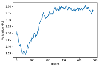
This graph is a bit difficult to see because of its large range and volatile nature. Let’s do something like this:

• Exclude the first 10 data points that are very different in scale from other parts of the curve.
• Replace each point with the exponential moving average of the previous point to get a smooth curve.

def smooth_curve(points, factor=0.9):
  smoothed_points = []
  for point in points:
    if smoothed_points:
      previous = smoothed_points[-1]
      smoothed_points.append(previous * factor + point * (1 - factor))
    else:
      smoothed_points.append(point)
  return smoothed_points

smooth_mae_history = smooth_curve(average_mae_history[10:])

plt.plot(range(1, len(smooth_mae_history) + 1), smooth_mae_history)
plt.xlabel('Epochs')
plt.ylabel('Validation MAE')
plt.show()

Looking at this graph, the verification MAE stopped decreasing after the 80th epoch. After this point, overfitting begins.

After tuning the other parameters of the model (you can adjust the size of the hidden layer as well as the number of epochs), use all the training data and train the model to be put into the final practice with the best parameters. Then check the performance with the test data:

model = build_model()

model.fit(train_data, train_targets,
          epochs=80, batch_size=16, verbose=0)
test_mse_score, test_mae_score = model.evaluate(test_data, test_targets)

test_mae_score