This post was written by referring to the contents of a deep learning book from the founder of Keras. : https://www.manning.com/books/deep-learning-with-python
Overfitting occurs when there are too few samples to learn. This is because you cannot train a generalizable model on new data. Given a lot of data, the model can learn all possible aspects of the data distribution. What if the number of data is small?
I recently created a model for predicting specific values using MLP. No matter how many layers were changed and K-fold verified, the Loss did not drop below 8. This was a limitation of the data. This can be solved by multiplying the data (I haven’t solved it yet, probably because it’s not image data).
Data augmentation
Data augmentation is a method of generating more training data from an existing training sample. This method increases the samples by applying several random transforms to produce a plausible image. The goal is to ensure that the model does not encounter exactly the same data twice when training. If the model learns several aspects of the data, it will help generalize.
In Keras, you can configure ImageDataGenerator to apply several kinds of random transforms to the images read. Let’s create an example first.
Before that, let’s download the data set from Kaggle in advance. : https://www.kaggle.com/c/dogs-vs-cats/data
from keras.preprocessing.image import ImageDataGenerator

datagen = ImageDataGenerator(
      rotation_range=40,
      width_shift_range=0.2,
      height_shift_range=0.2,
      shear_range=0.2,
      zoom_range=0.2,
      horizontal_flip=True,
      fill_mode='nearest')
There are a few more parameters (see Keras documentation). Let’s take a quick look at this code.
- rotation_range is the angular range to rotate the photo at random (between 0 and 80).
- width_shift_range and height_shift_range are the ranges to randomly translate the photo horizontally and vertically (ratio of the total width and height).
- shear_range is the angular range to apply the shear transformation at random.
- zoom_range is the range to zoom in on the photo at random.
- horizontal_flip randomly flips the image horizontally. Use when horizontal symmetry can be assumed (for example, landscape/portrait photography).
- fill_mode is a strategy to fill in pixels that need to be created newly due to rotation or horizontal/vertical movement.
Let’s look at a sample of the multiplied image:
from keras.preprocessing import image

fnames = sorted([os.path.join(train_cats_dir, fname) for fname in os.listdir(train_cats_dir)])

img_path = fnames[3]

img = image.load_img(img_path, target_size=(150, 150))

x = image.img_to_array(img)

x = x.reshape((1,) + x.shape)

i = 0
for batch in datagen.flow(x, batch_size=1):
    plt.figure(i)
    imgplot = plt.imshow(image.array_to_img(batch[0]))
    i += 1
    if i % 4 == 0:
        break

plt.show()
When training a new network using data proliferation, the same input data is not injected twice into the network. However, since it was created from a small number of original images, there is still a lot of correlation between the input data. In other words, new information cannot be created, only existing information can be recombined. That’s why it may not be enough to completely eliminate the overfitting. To further suppress overfitting, we will add a Dropout layer just before the fully connected classifier:
Let’s train this network using data proliferation and dropout:
model = models.Sequential()
model.add(layers.Conv2D(32, (3, 3), activation='relu',
                        input_shape=(150, 150, 3)))
model.add(layers.MaxPooling2D((2, 2)))
model.add(layers.Conv2D(64, (3, 3), activation='relu'))
model.add(layers.MaxPooling2D((2, 2)))
model.add(layers.Conv2D(128, (3, 3), activation='relu'))
model.add(layers.MaxPooling2D((2, 2)))
model.add(layers.Conv2D(128, (3, 3), activation='relu'))
model.add(layers.MaxPooling2D((2, 2)))
model.add(layers.Flatten())
model.add(layers.Dropout(0.5))
model.add(layers.Dense(512, activation='relu'))
model.add(layers.Dense(1, activation='sigmoid'))

model.compile(loss='binary_crossentropy',
              optimizer=optimizers.RMSprop(lr=1e-4),
              metrics=['acc'])
train_datagen = ImageDataGenerator(
    rescale=1./255,
    rotation_range=40,
    width_shift_range=0.2,
    height_shift_range=0.2,
    shear_range=0.2,
    zoom_range=0.2,
    horizontal_flip=True,)

test_datagen = ImageDataGenerator(rescale=1./255)

train_generator = train_datagen.flow_from_directory(

        train_dir,

        target_size=(150, 150),
        batch_size=32,

        class_mode='binary')

validation_generator = test_datagen.flow_from_directory(
        validation_dir,
        target_size=(150, 150),
        batch_size=32,
        class_mode='binary')

history = model.fit_generator(
      train_generator,
      steps_per_epoch=100,
      epochs=100,
      validation_data=validation_generator,
      validation_steps=50)
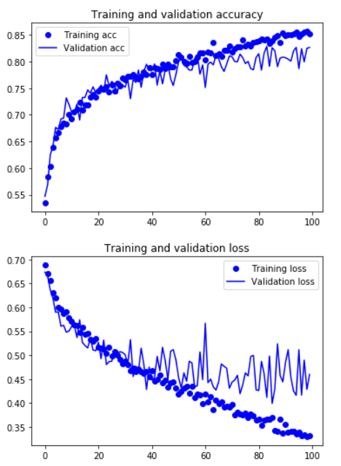
Let’s redraw the resulting graph:
import matplotlib.pyplot as plt
acc = history.history['acc']
val_acc = history.history['val_acc']
loss = history.history['loss']
val_loss = history.history['val_loss']

epochs = range(len(acc))

plt.plot(epochs, acc, 'bo', label='Training acc')
plt.plot(epochs, val_acc, 'b', label='Validation acc')
plt.title('Training and validation accuracy')
plt.legend()

plt.figure()

plt.plot(epochs, loss, 'bo', label='Training loss')
plt.plot(epochs, val_loss, 'b', label='Validation loss')
plt.title('Training and validation loss')
plt.legend()

plt.show()