Today, I’m going to cover an example of MLP (Muli-Layer Perceptron). For the concept of MLP, please refer to the article I wrote on December 8, 2019. Today, I am going to focus on practice rather than concept.
I want to use Kaggle data, which is famous for its dataset, but I want to use an advanced house price prediction dataset rather than the commonly known Boston house price dataset. Advancement means that the data I am trying to use has more characteristics and volumes. The data can be downloaded from the link below.
https://www.kaggle.com/c/house-prices-advanced-regression-techniques

Here’s a brief version of what you’ll find in the data description file.
- SalePrice – the property’s sale price in dollars. This is the target variable that you’re trying to predict.
- MSSubClass: The building class
- MSZoning: The general zoning classification
- LotFrontage: Linear feet of street connected to property
- LotArea: Lot size in square feet
- Street: Type of road access
- Alley: Type of alley access
- LotShape: General shape of property
- LandContour: Flatness of the property
- Utilities: Type of utilities available
- LotConfig: Lot configuration
- LandSlope: Slope of property
- Neighborhood: Physical locations within Ames city limits
- Condition1: Proximity to main road or railroad
- Condition2: Proximity to main road or railroad (if a second is present)
- BldgType: Type of dwelling
- HouseStyle: Style of dwelling
- OverallQual: Overall material and finish quality
- OverallCond: Overall condition rating
- YearBuilt: Original construction date
- YearRemodAdd: Remodel date
- RoofStyle: Type of roof
- RoofMatl: Roof material
- Exterior1st: Exterior covering on house
- Exterior2nd: Exterior covering on house (if more than one material)
- MasVnrType: Masonry veneer type
- MasVnrArea: Masonry veneer area in square feet
- ExterQual: Exterior material quality
- ExterCond: Present condition of the material on the exterior
- Foundation: Type of foundation
- BsmtQual: Height of the basement
- BsmtCond: General condition of the basement
- BsmtExposure: Walkout or garden level basement walls
- BsmtFinType1: Quality of basement finished area
- BsmtFinSF1: Type 1 finished square feet
- BsmtFinType2: Quality of second finished area (if present)
- BsmtFinSF2: Type 2 finished square feet
- BsmtUnfSF: Unfinished square feet of basement area
- TotalBsmtSF: Total square feet of basement area
- Heating: Type of heating
- HeatingQC: Heating quality and condition
- CentralAir: Central air conditioning
- Electrical: Electrical system
- 1stFlrSF: First Floor square feet
- 2ndFlrSF: Second floor square feet
- LowQualFinSF: Low quality finished square feet (all floors)
- GrLivArea: Above grade (ground) living area square feet
- BsmtFullBath: Basement full bathrooms
- BsmtHalfBath: Basement half bathrooms
- FullBath: Full bathrooms above grade
- HalfBath: Half baths above grade
- Bedroom: Number of bedrooms above basement level
- Kitchen: Number of kitchens
- KitchenQual: Kitchen quality
- TotRmsAbvGrd: Total rooms above grade (does not include bathrooms)
- Functional: Home functionality rating
- Fireplaces: Number of fireplaces
- FireplaceQu: Fireplace quality
- GarageType: Garage location
- GarageYrBlt: Year garage was built
- GarageFinish: Interior finish of the garage
- GarageCars: Size of garage in car capacity
- GarageArea: Size of garage in square feet
- GarageQual: Garage quality
- GarageCond: Garage condition
- PavedDrive: Paved driveway
- WoodDeckSF: Wood deck area in square feet
- OpenPorchSF: Open porch area in square feet
- EnclosedPorch: Enclosed porch area in square feet
- 3SsnPorch: Three season porch area in square feet
- ScreenPorch: Screen porch area in square feet
- PoolArea: Pool area in square feet
- PoolQC: Pool quality
- Fence: Fence quality
- MiscFeature: Miscellaneous feature not covered in other categories
- MiscVal: $Value of miscellaneous feature
- MoSold: Month Sold
- YrSold: Year Sold
- SaleType: Type of sale
- SaleCondition: Condition of sale
Upload Dataset
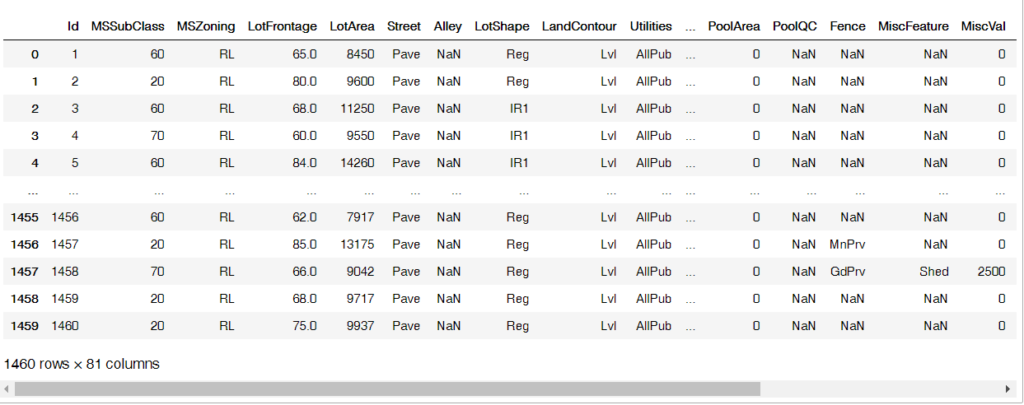
Let’s import the library and data.
import numpy as np
import pandas as pd

data = './train.csv'
raw_data = pd.read_csv(data)
raw_data
Data preprocessing
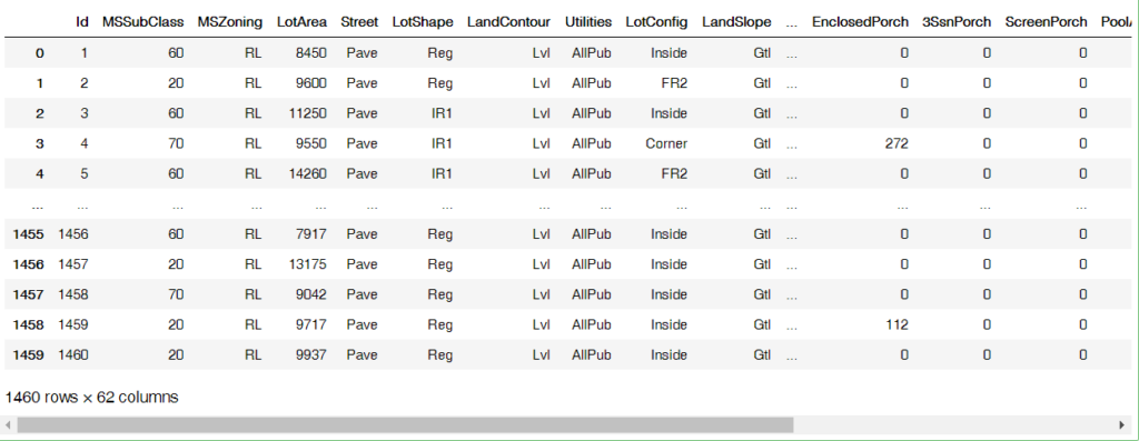
I deleted all columns with missing values.(NaN)
df_drop_column = raw_data.dropna(axis=1)
df_drop_column
In addition, feature data and target data were randomly created as follows among data having int values excluding data having object property.
X = df_drop_column[['LotArea','1stFlrSF','YearBuilt','GrLivArea','Fireplaces','GarageCars','GarageArea','PoolArea','MiscVal']]
y = df_drop_column[['SalePrice']]
Split training data and test data
It separates the data by importing the training data and test data division libraries from sklearn’s libraries. I divided it by 80% and 20% ratio, and check the shape of each data. This plays an important role in the dimension of the first input layer when constructing a neural network later.
from sklearn.model_selection import train_test_split

X_train, X_test, y_train, y_test = train_test_split(X, y, test_size=0.2, shuffle=True, random_state=1002)
print(X_train.shape)
print(X_test.shape)
print(y_train.shape)
print(y_test.shape)
X_train.shape[1]
Data normalization
If the range of input data is different, training may not work well when training a neural network. Therefore, normalization of data proceeds as follows.
mean = X_train.mean(axis=0)
X_train -= mean
std = X_train.std(axis=0)
X_train /= std

X_test -= mean
X_test /= std
Creating the model
from keras import models
from keras import layers
It measures MAE (the absolute value of the predicted value and the distance of the target data), but if the MAE is 0.5, there will be a difference of about 500 dollars.
def build_model():
    model = models.Sequential()
    model.add(layers.Dense(64, activation='relu',
                           input_shape=(X_train.shape[1],)))
    model.add(layers.Dense(64, activation='relu'))
    model.add(layers.Dense(1))
    model.compile(optimizer='rmsprop', loss='mse', metrics=['mae'])
    return model
Training validation using k-fold cross validation
A method of dividing the data into k (about 4-5) partitions, creating k models each, training in k-1 partitions, and evaluating in the remaining partitions
k = 4
num_val_samples = len(X_train) // k
num_epochs = 100
all_scores = []
for i in range(k):
    print('processing fold #', i)
    val_data = X_train[i * num_val_samples: (i + 1) * num_val_samples]
    val_targets = y_train[i * num_val_samples: (i + 1) * num_val_samples]

    partial_train_data = np.concatenate(
        [X_train[:i * num_val_samples],
         X_train[(i + 1) * num_val_samples:]],axis=0)
    partial_train_targets = np.concatenate(
        [y_train[:i * num_val_samples],
         y_train[(i + 1) * num_val_samples:]],axis=0)

    model = build_model()

    model.fit(partial_train_data, partial_train_targets,
              epochs=num_epochs, batch_size=1, verbose=0)

    val_mse, val_mae = model.evaluate(val_data, val_targets, verbose=0)
    all_scores.append(val_mae)
Check MAE score
all_scores

np.mean(all_scores)
Saving validation scores at each fold in log
from keras import backend as K

K.clear_session()
num_epochs = 500
all_mae_histories = []
for i in range(k):
    print('processing fold #', i)

    val_data = X_train[i * num_val_samples: (i + 1) * num_val_samples]
    val_targets = y_train[i * num_val_samples: (i + 1) * num_val_samples]

    partial_train_data = np.concatenate(
        [X_train[:i * num_val_samples],
         X_train[(i + 1) * num_val_samples:]],
        axis=0)
    partial_train_targets = np.concatenate(
        [y_train[:i * num_val_samples],
         y_train[(i + 1) * num_val_samples:]],
        axis=0)

    model = build_model()

    history = model.fit(partial_train_data, partial_train_targets,
                        validation_data=(val_data, val_targets),
                        epochs=num_epochs, batch_size=1, verbose=0)
    mae_history = history.history['val_mean_absolute_error']
    all_mae_histories.append(mae_history)
Calculate epoch’s MAE average score for all folds
average_mae_history = [np.mean([x[i] for x in all_mae_histories]) for i in range(num_epochs)]
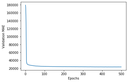
Display verification score graph
import matplotlib.pyplot as plt

plt.plot(range(1, len(average_mae_history) + 1), average_mae_history)
plt.xlabel('Epochs')
plt.ylabel('Validation MAE')
plt.show()
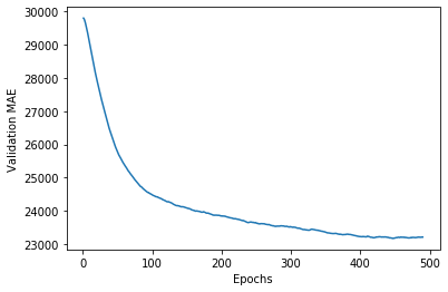
def smooth_curve(points, factor=0.9):
  smoothed_points = []
  for point in points:
    if smoothed_points:
      previous = smoothed_points[-1]
      smoothed_points.append(previous * factor + point * (1 - factor))
    else:
      smoothed_points.append(point)
  return smoothed_points

smooth_mae_history = smooth_curve(average_mae_history[10:])

plt.plot(range(1, len(smooth_mae_history) + 1), smooth_mae_history)
plt.xlabel('Epochs')
plt.ylabel('Validation MAE')
plt.show()
Training the final model
model = build_model()

model.fit(X_train, y_train,
          epochs=80, batch_size=16, verbose=0)
test_mse_score, test_mae_score = model.evaluate(X_test, y_test)

test_mae_score
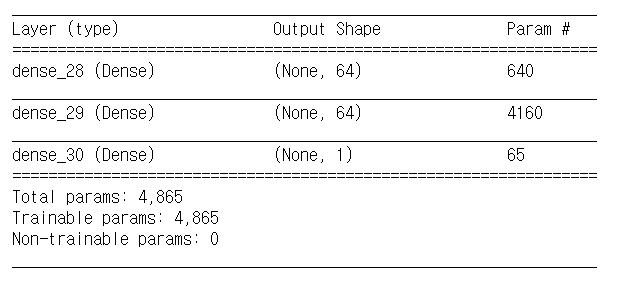
Summary of model information
model.summary()
Evaluate model accuracy
model.evaluate(X_test, y_test, batch_size=32)
Output random predictions
model.predict(X_input, batch_size=32)
Saving model
model.save("model_name.h5")
Loading model
from tensorflow.keras.models import load_model
model = load_model("model_name.h5")
You can find this full code in github!
https://github.com/maker-hong/Deep-Learning/blob/master/200810_MLP_example_code_predicting_house_prices.ipynb